Prepare data for the analysis • SDMtune

Intro

In this article you will learn how to prepare the data to train models using SDMtune. We will use the virtualSp dataset included in the package and environmental predictors from the WorldClim dataset.

Set working environment

Load the required packages for the analysis:

library(ggplot2)    # To plot locations
library(maps)       # To access useful maps
library(rasterVis)  # To plot raster objects

Acquire environmental variables

For the analysis we use the climate data of WorldClim version 1.4 (Hijmans et al. 2005) and the terrestrial ecoregions from WWF (Olson et al. 2001) included in the dismo package:

files <- list.files(path = file.path(system.file(package = "dismo"), "ex"),
                    pattern = "grd",
                    full.names = TRUE)

We convert the files in a raster object that will be used later in the analysis:

predictors <- terra::rast(files)

There are nine environmental variables, eight continuous and one categorical:

names(predictors)
#> [1] "bio1"  "bio12" "bio16" "bio17" "bio5"  "bio6"  "bio7"  "bio8"  "biome"

Continuous variables
- bio1 Annual Mean Temperature
- bio5 Max Temperature of Warmest Month
- bio6 Min Temperature of Coldest Month
- bio7 Temperature Annual Range (bio5-bio6)
- bio8 Mean Temperature of Wettest Quarter
- bio12 Annual Precipitation
- bio16 Precipitation of Wettest Quarter
- bio17 Precipitation of Driest Quarter
Categorical variables
- biome Terrestrial Ecoregions of the World

We can plot bio1 using the gplot function from the rasterVis package:

gplot(predictors$bio1) +
    geom_tile(mapping = aes(fill = value)) +
    coord_equal() +
    scale_fill_gradientn(colours = c("#2c7bb6", "#abd9e9", "#ffffbf", "#fdae61", "#d7191c"),
                         na.value = "transparent",
                         name = "°C x 10") +
    labs(title = "Annual Mean Temperature",
         x = "longitude",
         y = "latitude") +
    scale_x_continuous(expand = c(0, 0)) +
    scale_y_continuous(expand = c(0, 0)) +
    theme_minimal() +
    theme(plot.title = element_text(hjust = 0.5),
          axis.ticks.x = element_blank(),
          axis.ticks.y = element_blank())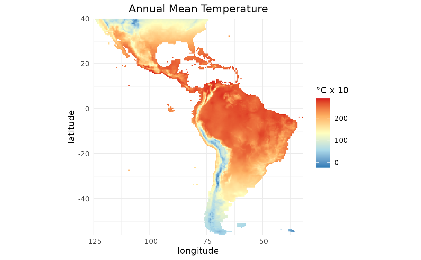

Prepare presence and background locations

Let’s load the SDMtune package:

library(SDMtune)
#> 
#>    _____  ____   __  ___ __
#>   / ___/ / __ \ /  |/  // /_ __  __ ____   ___
#>   \__ \ / / / // /|_/ // __// / / // __ \ / _ \
#>  ___/ // /_/ // /  / // /_ / /_/ // / / //  __/
#> /____//_____//_/  /_/ \__/ \__,_//_/ /_/ \___/  version 1.3.1
#> 
#> To cite this package in publications type: citation("SDMtune").

For demonstrating how to use SDMtune we use the random generated virtual species virtualSp dataset included in the package. The dataset contains 400 coordinates for presence and 5000 for background locations.

help(virtualSp)
p_coords <- virtualSp$presence
bg_coords <- virtualSp$background

Plot the study area together with the presence locations:

ggplot(data = map_data("world"), mapping = aes(x = long, y = lat)) +
    geom_polygon(aes(group = group), fill = "grey95", color = "gray40", size = 0.2) +
    geom_jitter(data = p_coords, aes(x = x, y = y), color = "red",
                alpha = 0.4, size = 1) +
    labs(x = "longitude", y = "latitude") +
    theme_minimal() +
    theme(legend.position = "none") +
    coord_fixed() +
    scale_x_continuous(limits = c(-125, -32)) +
    scale_y_continuous(limits = c(-56, 40))
#> Warning: Using `size` aesthetic for lines was deprecated in ggplot2 3.4.0.
#> ℹ Please use `linewidth` instead.
#> This warning is displayed once every 8 hours.
#> Call `lifecycle::last_lifecycle_warnings()` to see where this warning was
#> generated.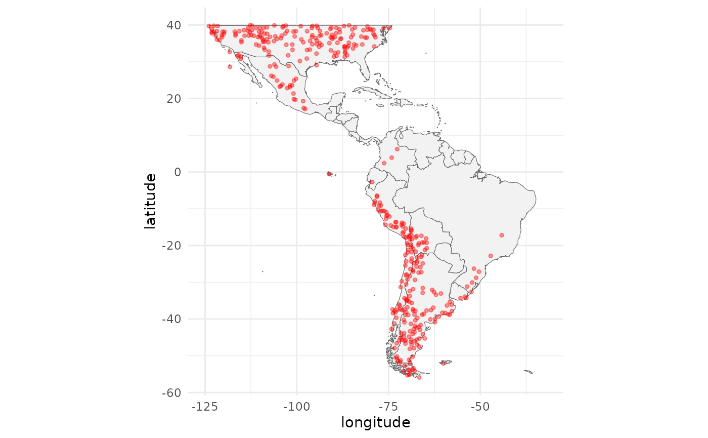

To plot the background locations run the following code:

ggplot(data = map_data("world"), mapping = aes(x = long, y = lat)) +
    geom_polygon(aes(group = group), fill = "grey95", color = "gray40", size = 0.2) +
    geom_jitter(data = as.data.frame(bg_coords), aes(x = x, y = y),
                color = "blue", alpha = 0.4, size = 0.5) +
    labs(x = "longitude", y = "latitude") +
    theme_minimal() +
    theme(legend.position = "none") +
    coord_fixed() +
    scale_x_continuous(limits = c(-125, -32)) +
    scale_y_continuous(limits = c(-56, 40))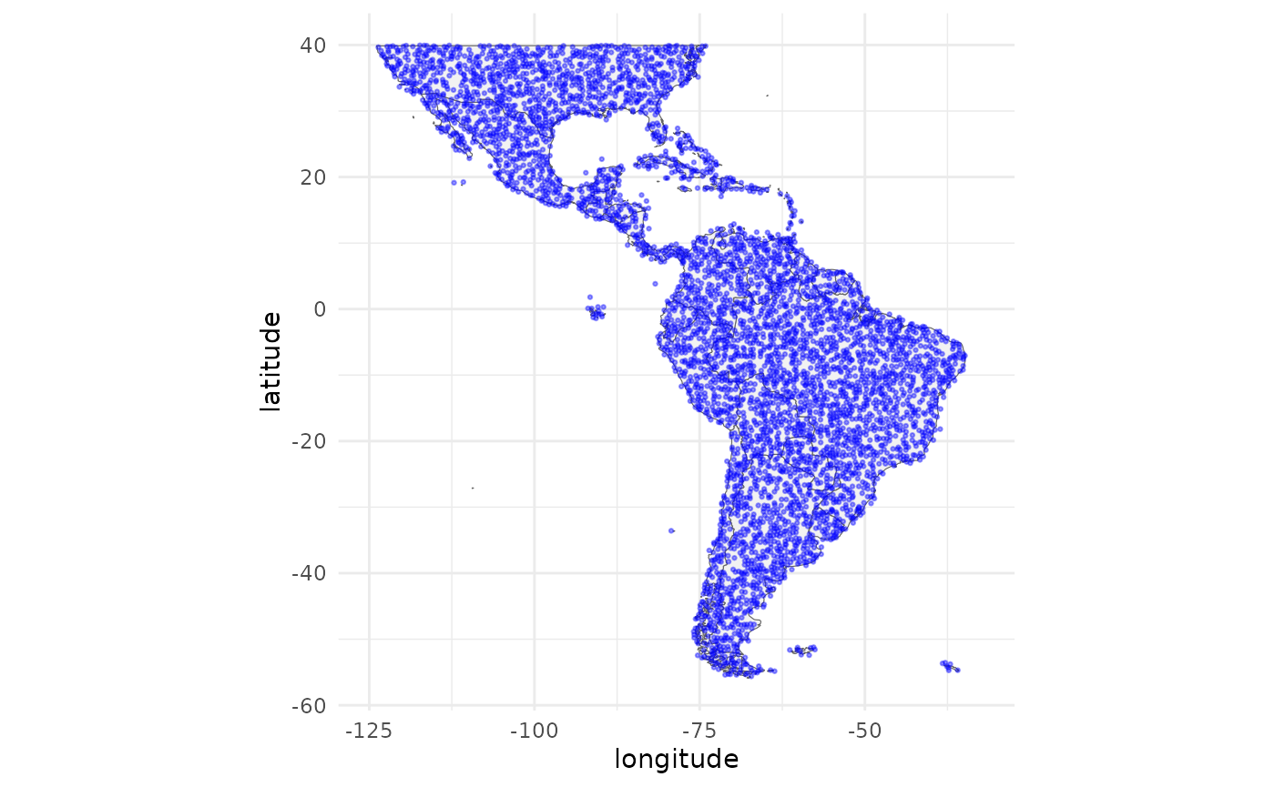

Create an SWD object

Before training a model we have to prepare the data in the correct format. The prepareSWD() function creates an SWD() object that stores the species name, the coordinates of the species at presence and absence/background locations and the value of the environmental variables at the locations. The argument categorical indicates which environmental variables are categorical. In our example biome is categorical (we can pass a vector if we have more than one categorical environmental variable). The function extracts the value of the environmental variables for each location and excludes those locations that have NA value for at least one environmental variable.

data <- prepareSWD(species = "Virtual species",
                   p = p_coords,
                   a = bg_coords,
                   env = predictors,
                   categorical = "biome")

Explore the SWD object

Let’s have a look at the created SWD() object:

data
#> 
#> ── Object of class: <SWD> ──
#> 
#> ── Info
#> • Species: Virtual species
#> • Presence locations: 400
#> • Absence locations: 5000
#> 
#> ── Variables
#> • Continuous: "bio1", "bio12", "bio16", "bio17", "bio5", "bio6", "bio7", and
#> "bio8"
#> • Categorical: "biome"

When we print an SWD() object we get a bunch of information:

the name of the class;
the name of the species;
the number of presence locations;
the number of absence/background locations;
the environmental variables available in the dataset:
- the name of the continuous environmental variables, if any;
- the name of the categorical environmental variables, if any.

The object contains four slots: @species, @coords @data and @pa. @pa contains a vector with 1 for presence and 0 for absence/background locations. To visualize the data we run:

head(data@data)

bio1	bio12	bio16	bio17	bio5	bio6	bio7	bio8	biome
32	59	55	0	152	-118	270	66	10
161	1427	426	275	323	-10	333	78	4
156	977	341	137	342	-41	384	203	8
119	975	305	177	313	-77	390	190	8
112	633	268	42	333	-106	440	218	8
92	196	64	37	254	-37	291	26	8

We can visualize the coordinates with:

head(data@coords)

X	Y
-67.75	-21.75
-86.75	33.75
-96.25	35.75
-89.25	39.25
-98.75	39.75
-68.75	-41.25

or the name of the species with:

data@species
#> [1] "Virtual species"

Save an SWD object

We can save the SWD() object in a .csv file using the function swd2csv() (the function saves the file in the working directory). There are two possibilities:

save the object in a single file with the column pa indicating if the location is a presence (1) or an absence/background (0) site

swd2csv(data, file_name = "data.csv")

save the object in two separate files: one for the presence and the other for the absence/background locations

swd2csv(data, file_name = c("presence.csv", "background.csv"))

Conclusion

In this article you have learned:

how to create a raster object;
how to plot a raster object using the gplot function included in the rasterVis package;
how to plot locations using the ggplot and the maps packages;
how to create an SWD() objects;
how to extract information from an SWD() object;
how to save an SWD() object in a .csv file.

Move on to the second article and learn how to train models using SDMtune.

References

Hijmans, Robert J., Susan E. Cameron, Juan L. Parra, Peter G. Jones, and Andy Jarvis. 2005. “Very High Resolution Interpolated Climate Surfaces for Global Land Areas.” International Journal of Climatology 25 (15): 1965–78. https://doi.org/https://doi.org/10.1002/joc.1276.

Olson, David M., Eric Dinerstein, Eric D. Wikramanayake, Neil D. Burgess, George V. N. Powell, Emma C. Underwood, Jennifer A. D’amico, et al. 2001. “Terrestrial Ecoregions of the World: A New Map of Life on Earth.” BioScience 51 (11): 933. https://doi.org/10.1641/0006-3568(2001)051[0933:TEOTWA]2.0.CO;2.