Plot Response Curve

Plot the Response Curve of the given environmental variable.

Usage

plotResponse(
  model,
  var,
  type = NULL,
  only_presence = FALSE,
  marginal = FALSE,
  fun = mean,
  rug = FALSE,
  color = "red"
)

Arguments

model

SDMmodel or SDMmodelCV object.

var

character. Name of the variable to be plotted.

type

character. The output type used for "Maxent" and "Maxnet" methods, possible values are "cloglog" and "logistic".

only_presence

logical. If TRUE it uses only the presence locations when applying the function for the marginal response.

marginal

logical. If TRUE it plots the marginal response curve.

fun

function used to compute the level of the other variables for marginal curves.

rug

logical. If TRUE it adds the rug plot for the presence and absence/background locations, available only for continuous variables.

color

The color of the curve, default is "red".

Value

A ggplot object.

Details

• Note that fun is not a character argument, you must use mean and not "mean".

• If you want to modify the plot, first you have to assign the output of the function to a variable, and then you have two options:

  • Modify the ggplot object by editing the theme or adding additional elements

  • Get the data with ggplot2::ggplot_build() and then build your own plot (see examples)

Author

Sergio Vignali

Examples

# Acquire environmental variables
files <- list.files(path = file.path(system.file(package = "dismo"), "ex"),
                    pattern = "grd",
                    full.names = TRUE)

predictors <- terra::rast(files)

# Prepare presence and background locations
p_coords <- virtualSp$presence
bg_coords <- virtualSp$background

# Create SWD object
data <- prepareSWD(species = "Virtual species",
                   p = p_coords,
                   a = bg_coords,
                   env = predictors,
                   categorical = "biome")
#> ℹ Extracting predictor information for presence locations
#> ✔ Extracting predictor information for presence locations [39ms]
#> 
#> ℹ Extracting predictor information for absence/background locations
#> ✔ Extracting predictor information for absence/background locations [66ms]
#> 

# Train a model
model <- train(method = "Maxnet",
               data = data,
               fc = "lq")

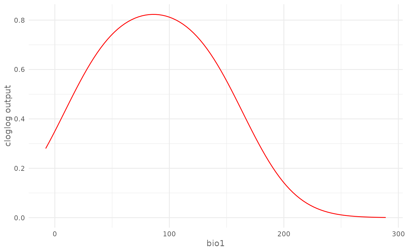
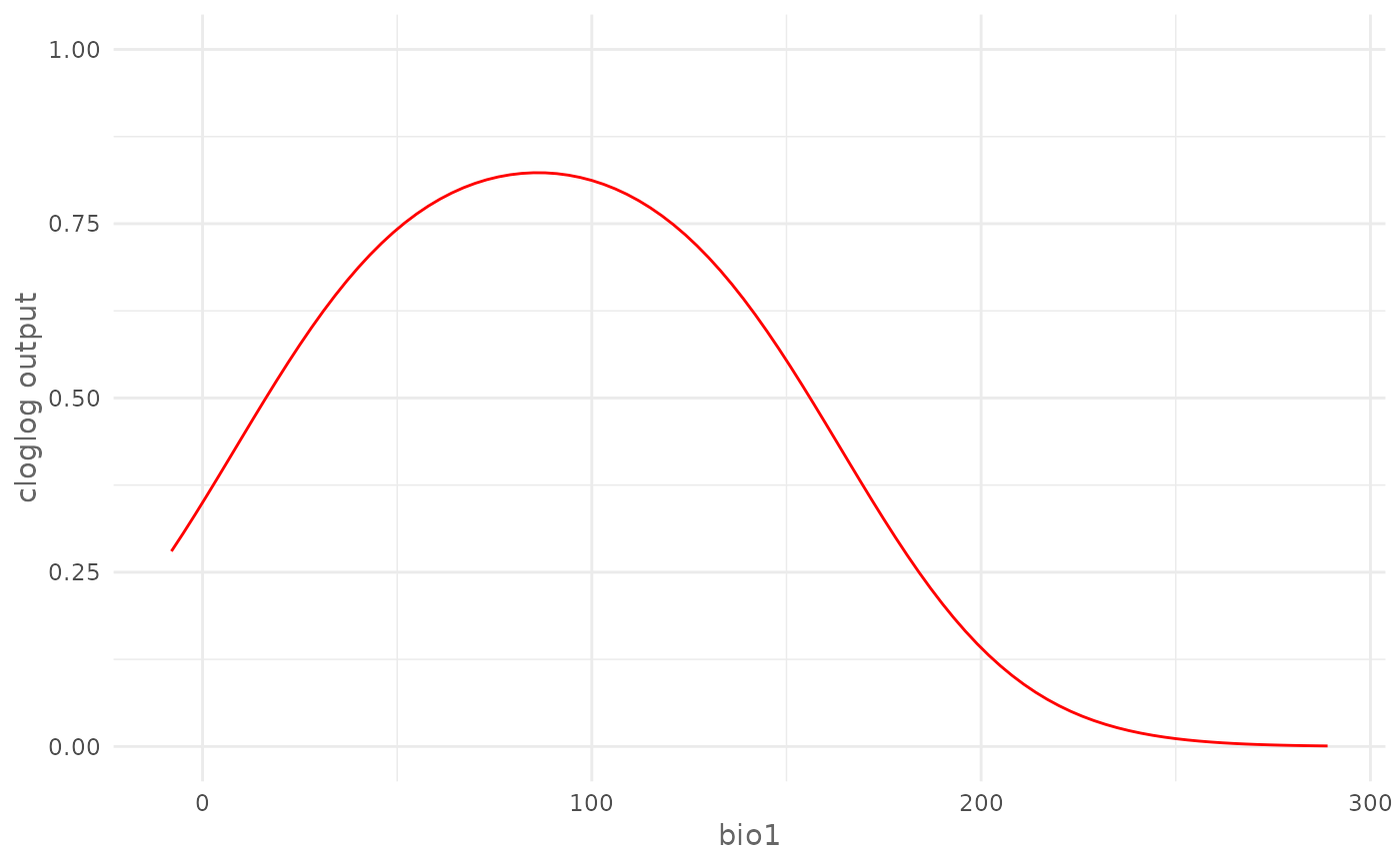
# Plot cloglog response curve for a continuous environmental variable (bio1)
plotResponse(model,
             var = "bio1",
             type = "cloglog")


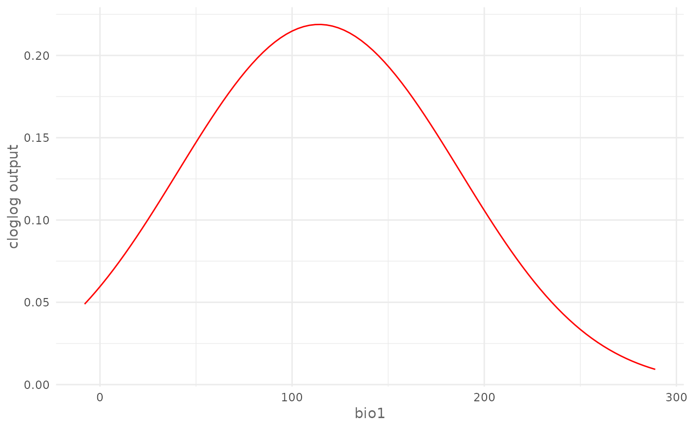
# Plot marginal cloglog response curve for a continuous environmental
# variable (bio1)
plotResponse(model,
             var = "bio1",
             type = "cloglog",
             marginal = TRUE)


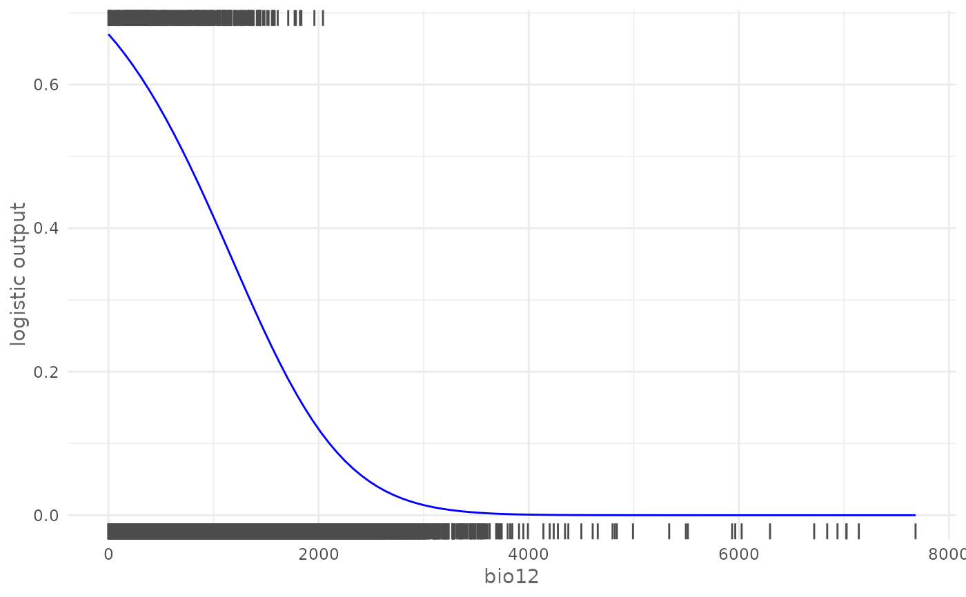
# Plot logistic response curve for a continuous environmental variable
# (bio12) adding the rugs and giving a custom color
plotResponse(model,
             var = "bio12",
             type = "logistic",
             rug = TRUE,
             color = "blue")


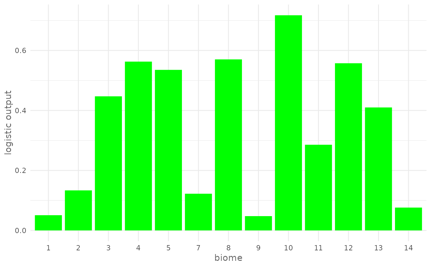
# Plot response curve for a categorical environmental variable (biome) giving
# a custom color
plotResponse(model,
             var = "biome",
             type = "logistic",
             color = "green")


# Modify plot
# Change y axes limits
my_plot <- plotResponse(model,
                        var = "bio1",
                        type = "cloglog")
my_plot +
  ggplot2::scale_y_continuous(limits = c(0, 1))


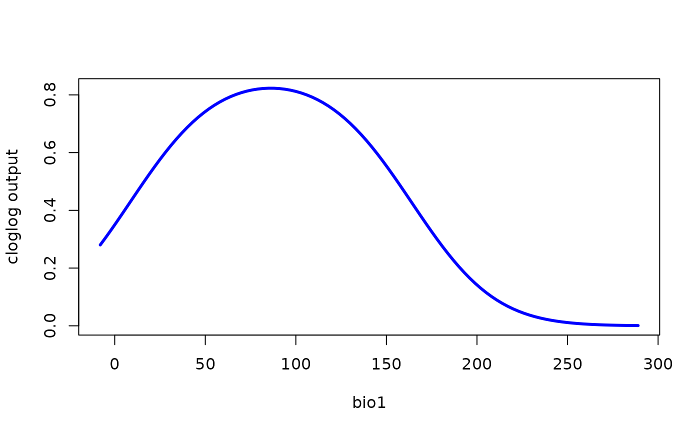
# Get the data and create your own plot:
df <- ggplot2::ggplot_build(my_plot)$data[[1]]
plot(df$x, df$y,
     type = "l",
     lwd = 3,
     col = "blue",
     xlab = "bio1",
     ylab = "cloglog output")


# Train a model with cross validation
folds <- randomFolds(data,
                     k = 4,
                     only_presence = TRUE)

model <- train(method = "Maxnet",
               data = data,
               fc = "lq",
               folds = folds)

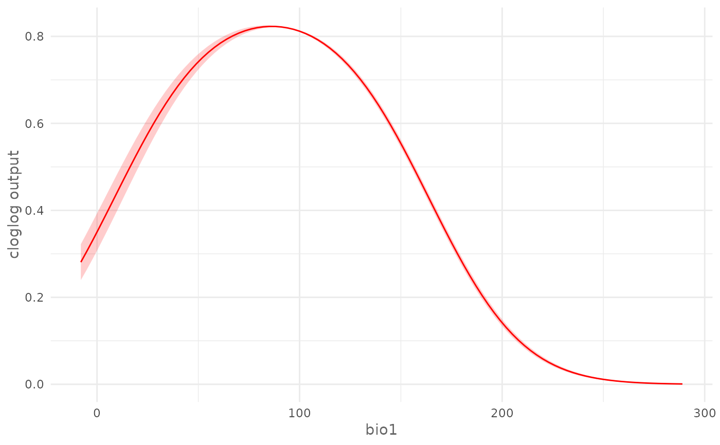
# Plot cloglog response curve for a continuous environmental variable (bio17)
plotResponse(model,
             var = "bio1",
             type = "cloglog")


# Plot logistic response curve for a categorical environmental variable
# (biome) giving a custom color
plotResponse(model,
             var = "biome",
             type = "logistic",
             color = "green")