Train presence absence models • SDMtune

Intro

All the previous articles are based on presence only methods, in this article you will learn how to train a presence absence model. The following examples are based on the Artificial Neural Networks method (Venables and Ripley 2002), but you can adapt the code for any of the other supported methods.

Prepare the data for the analysis

We use the first 8 environmental variables and the same virtualSp() dataset selecting the absence instead of the background locations.

p_coords <- virtualSp$presence
a_coords <- virtualSp$absence

data <- prepareSWD(species = "Virtual species", 
                   p = p_coords, 
                   a = a_coords, 
                   env = predictors[[1:8]])

data

#> 
#> ── Object of class: <SWD> ──
#> 
#> ── Info
#> • Species: Virtual species
#> • Presence locations: 400
#> • Absence locations: 300
#> 
#> ── Variables
#> • Continuous: "bio1", "bio12", "bio16", "bio17", "bio5", "bio6", "bio7", and
#> "bio8"
#> • Categorical: NA

There are 400 presence and 300 absence locations.

For the model evaluation we will create a training and testing datasets, holding apart 20% of the data:

library(zeallot)
c(train, test) %<-% trainValTest(data, 
                                 test = 0.2, 
                                 seed = 25)

At this point we have 560 training and 140 testing locations. We create a 4-folds partition to run cross validation:

folds <- randomFolds(train, 
                     k = 4, 
                     seed = 25)

Train the model

We first train the model with default settings and 10 neurons:

set.seed(25)
model <- train("ANN", 
               data = train, 
               size = 10, 
               folds = folds)
model
#> 
#> ── Object of class: <SDMmodelCV> ──
#> 
#> Method: Artificial Neural Networks
#> 
#> ── Hyperparameters
#> • size: 10
#> • decay: 0
#> • rang: 0.7
#> • maxit: 100
#> 
#> ── Info
#> • Species: Virtual species
#> • Replicates: 4
#> • Total presence locations: 320
#> • Total absence locations: 240
#> 
#> ── Variables
#> • Continuous: "bio1", "bio12", "bio16", "bio17", "bio5", "bio6", "bio7", and
#> "bio8"
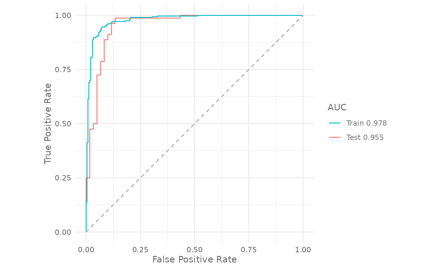
#> • Categorical: NA

Let’s check the training and testing AUC:

auc(model)
#> [1] 0.8180469
auc(model, test = TRUE)
#> [1] 0.7931771

Tune model hyperparameters

To check which hyperparameters can be tuned we use the function getTunableArgs() function:

getTunableArgs(model)
#> [1] "size"  "decay" "rang"  "maxit"

We use the function optimizeModel() to tune the hyperparameters:

h <- list(size = 10:50, 
          decay = c(0.01, 0.05, 0.1, 0.2, 0.3, 0.4, 0.5),
          maxit = c(50, 100, 300, 500))

om <- optimizeModel(model, 
                    hypers = h, 
                    metric = "auc", 
                    seed = 25)

The best model is:

best_model <- om@models[[1]]
om@results[1, ]

size	decay	rang	maxit	train_AUC	test_AUC	diff_AUC
16	0.4	0.7	500	0.9853791	0.9545833	0.0307957

The validation AUC increased from 0.7931771 of the default models to 0.9545833 of the optimized one.

Evaluate the final model

We now train a model with the same configuration as found by the function optimizeModel() without cross validation (i.e. using all presence and background locations) and we evaluate it using the held apart testing dataset:

set.seed(25)
final_model <- combineCV(om@models[[1]])

plotROC(final_model, 
        test = test)
#> Warning: The following aesthetics were dropped during statistical transformation: m, d
#> ℹ This can happen when ggplot fails to infer the correct grouping structure in
#>   the data.
#> ℹ Did you forget to specify a `group` aesthetic or to convert a numerical
#>   variable into a factor?

Conclusion

In this tutorial you have learned a general way to train, evaluate and tune model using Artificial Neural Network, but you can apply the same workflow to other methods.

References

Venables, W N, and B. D. Ripley. 2002. Modern Applied Statistics with S. Fourth Edi. New York, NY: Springer.