Tune model hyperparameters • SDMtune

Intro

In the previous articles you have learned the core functions of SDMtune and how to perform data-driven variable selection. In this article you will learn how to tune the model hyperparameters.

Training, validation and testing split

When you tune the model hyperparameters you iteratively adjust the hyperparameters while monitoring the changes in the evaluation metric computed using the testing dataset. In this process, the information contained in the testing dataset leaks in the model and therefore, at the end of the process, the testing dataset doesn’t represent anymore an independent set to evaluate the model Chollet and Allaire (2018). A better strategy, than splitting the observation locations in training and testing, would be to split them into training, validation and testing datasets. The training dataset is then used to train the model, the validation datasets to drive the hyperparameter tuning and the testing dataset to evaluate the tuned model. The function trainValTest() allows to split the data in three folds containing the provided percentage of data. For illustration purpose let’s split the presence locations in training (60%), validation (20%) and testing (20%) datasets:

library(zeallot)  # For unpacking assignment
c(train, val, test) %<-% trainValTest(data, 
                                      val = 0.2, 
                                      test = 0.2, 
                                      only_presence = TRUE, 
                                      seed = 61516)

cat("# Training  : ", nrow(train@data))
#> # Training  :  5240
cat("# Validation: ", nrow(val@data))
#> # Validation:  5080
cat("# Testing   : ", nrow(test@data))
#> # Testing   :  5080

We now train a Maxnet model with default settings and using the training dataset:

model <- train("Maxnet", 
               data = train)

Another approach would be to split the data in two folds: training and testing, use the cross validation strategy with the training dataset to tune the model hyperparameters, and evaluate the tuned model with the unseen held apart testing dataset. For execution time reason we demonstrate the first approach but you are free to try out the second one.

Check the effect of varying one hyperparameter

To see the effect of varying one hyperparameter on the model performance we can use the function gridSearch(). The function iterates through a set of predefined hyperparameter values, train the model and displays in real-time the evaluation metric in the RStudio viewer pane (hover over the points to get a tooltip with extra information). Let’s see how the AUC changes varying the regularization multiplier. First we have to define the values for the hyperparameter that we want to test. For that we create a named list that we will use as an argument for the function gridSearch():

# Define the values for the regularization multiplier
h <- list(reg = seq(0.2, 1, 0.1))

# Call the gridSearch function
exp_1 <- gridSearch(model, 
                    hypers = h, 
                    metric = "auc", 
                    test = val)

As you noticed we used the validation dataset as test argument. The output of the function is an object of class SDMtune(). Let’s print it:

exp_1
#> 
#> ── Object of class: <SDMtune> ──
#> 
#> Method: Maxnet
#> 
#> ── Tested hyperparameters
#> • fc: "lqph"
#> • reg: 0.2, 0.3, 0.4, 0.5, 0.6, 0.7, 0.8, 0.9, and 1

When you print the output, the text contains the models configuration that have been used during the execution of the function. In our case, only the regularization multiplier reg has multiple values. You can plot the SDMtune() object:

plot(exp_1, 
     title = "Experiment 1")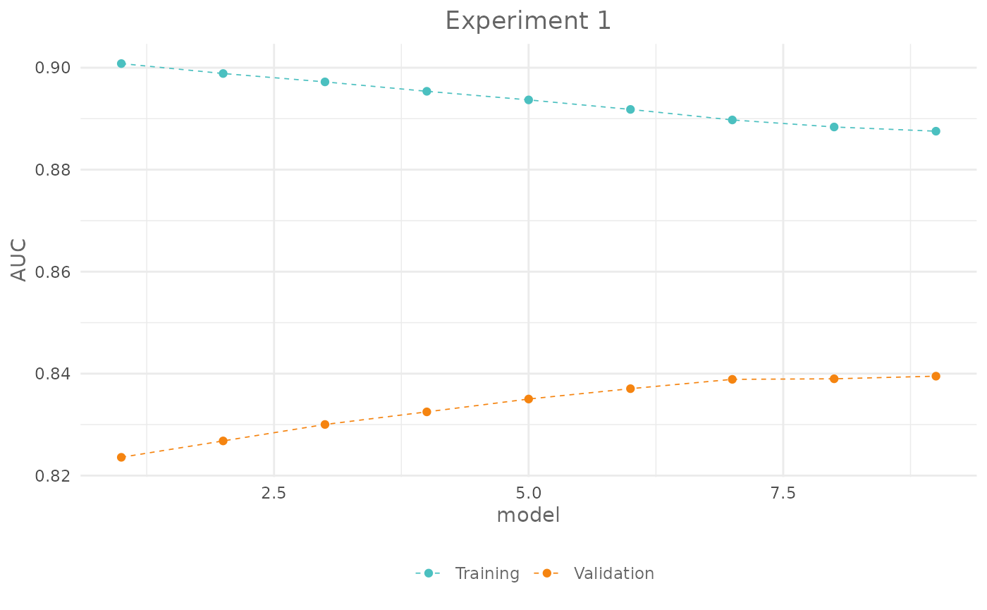

and you can also recreate the interactive chart using:

plot(exp_1, 
     title = "Experiment 1", 
     interactive = TRUE)

The SDMtune() object stores the results in the slot @results:

exp_1@results

fc	reg	train_AUC	test_AUC	diff_AUC
lqph	0.2	0.9008033	0.8235925	0.0772108
lqph	0.3	0.8988542	0.8268050	0.0720492
lqph	0.4	0.8972125	0.8300300	0.0671825
lqph	0.5	0.8953675	0.8325025	0.0628650
lqph	0.6	0.8936800	0.8350225	0.0586575
lqph	0.7	0.8918142	0.8370500	0.0547642
lqph	0.8	0.8897492	0.8388800	0.0508692
lqph	0.9	0.8883683	0.8389875	0.0493808
lqph	1.0	0.8875433	0.8395025	0.0480408

You can order them with:

exp_1@results[order(-exp_1@results$test_AUC), ]

	fc	reg	train_AUC	test_AUC	diff_AUC
9	lqph	1.0	0.8875433	0.8395025	0.0480408
8	lqph	0.9	0.8883683	0.8389875	0.0493808
7	lqph	0.8	0.8897492	0.8388800	0.0508692
6	lqph	0.7	0.8918142	0.8370500	0.0547642
5	lqph	0.6	0.8936800	0.8350225	0.0586575
4	lqph	0.5	0.8953675	0.8325025	0.0628650
3	lqph	0.4	0.8972125	0.8300300	0.0671825
2	lqph	0.3	0.8988542	0.8268050	0.0720492
1	lqph	0.2	0.9008033	0.8235925	0.0772108

Try yourself

Try to see how TSS changes varying the regularization multiplier from 1 to 4 (highlight to see the solution):

# Define the values for reg
h <- list(reg = 1:4)

# Call the gridSearch function
exp_2 <- gridSearch(model, 
                    hypers = h, 
                    metric = "tss", 
                    test = val)

and how AUC changes varying the feature combinations using the following values: l, lq, lh, lqp, lqph and lqpht (highlight to see the solution):

# Define the values for fc
h <- list(fc = c("l", "lq", "lh", "lqp", "lqph", "lqpht"))

# Call the gridSearch function
exp_3 <- gridSearch(model, 
                    hypers = h, 
                    metric = "auc", 
                    test = val)

Train a Maxent model and see how the AUC changes varying the number of iterations from 300 to 1100 with increments of 200 (highlight to see the solution):

maxent_model <- train("Maxent", 
                      data = data)

# Define the values for fc
h <- list("iter" = seq(300, 1100, 200))

# Call the gridSearch function
exp_4 <- gridSearch(maxent_model, 
                    hypers = h, 
                    metric = "auc", 
                    test = val)

To see which hyperparameters can be tuned in a given model use the function getTunableArgs(). For example:

getTunableArgs(model)
#> [1] "fc"  "reg"

Tune hyperparameters

To tune the model hyperparameters you should run all the possible combinations of hyperparameters. Here is an example using combinations of regularization multiplier and feature classes:

h <- list(reg = seq(0.2, 2, 0.2), 
          fc = c("l", "lq", "lh", "lqp", "lqph", "lqpht"))

exp_5 <- gridSearch(model, 
                    hypers = h, 
                    metric = "auc", 
                    test = val)

This code takes already quite long as it has to train 60 models. Imagine if you want to check more values for the regularization multiplier and maybe add the number of iterations (in the case of a Maxent model). The number of models to be trained increases exponentially and consequently the execution time. In the next two paragraphs we will present two possible alternative to the gridSearch() function.

Random search

The function randomSearch() trains models taking a random sample of the predefined configurations. In the next example we select 10 random configurations:

h <- list(reg = seq(0.2, 5, 0.2), 
          fc = c("l", "lq", "lh", "lp", "lqp", "lqph"))

exp_6 <- randomSearch(model, 
                      hypers = h, 
                      metric = "auc", 
                      test = val, 
                      pop = 10, 
                      seed = 65466)

The real-time chart plots two different graphs, one with the chosen metric for each trained model and one with the evaluation metric for the starting and the best found model. As you can see, the function is able to find a better combination of the model hyperparameters compared to the starting model; and this training only 10 instead of 150 models. The results includes the 10 trained model. If you are not happy with the solution, you can check the best hyperparameter combinations and this gives you an intuition of which ones are the hyperparameters to “refine” using the function gridSearch(). The SDMtune() object stores the results in a data.frame than can be accessed with the following command:

exp_6@results

fc	reg	train_AUC	test_AUC	diff_AUC
lp	2.2	0.8691417	0.8482400	0.0209017
lp	0.8	0.8734875	0.8472100	0.0262775
lqph	3.2	0.8713750	0.8435500	0.0278250
lqph	2.4	0.8764117	0.8435025	0.0329092
lq	3.8	0.8597967	0.8419325	0.0178642
lh	3.2	0.8698442	0.8414150	0.0284292
lqph	1.2	0.8854808	0.8408300	0.0446508
lh	2.0	0.8751675	0.8399250	0.0352425
lh	1.0	0.8860650	0.8391100	0.0469550
l	0.4	0.8489625	0.8269575	0.0220050

Optimize Model

The previous function doesn’t learn anything from the trained models, it just selects n random combinations of hyperparameters. The function optimizeModel() uses a genetic algorithm to find an optimum or near optimum solution. Check the function documentation to understand how it works, here we provide the code to execute it:

exp_7 <- optimizeModel(model, 
                       hypers = h, 
                       metric = "auc", 
                       test = val, 
                       pop = 15, 
                       gen = 2, 
                       seed = 798)

Evaluate final model

Let’s say we want to use the best tuned model found by the randomSearch() function. Before evaluating the model using the testing dataset, we can merge the training and the validation datasets together to increase the number of locations and train a new model with the merged observations and the tuned configuration. At this point we may have removed variables using the varSel() or reduceVar() function. If this is the case, we cannot merge directly the initial datasets which contain all the environmental variables. We can extract the train dataset with the selected variables from the output of the experiment and merge it with the validation dataset using the function mergeSWD():

# Index of the best model in the experiment
index <- which.max(exp_6@results$test_AUC)

# New train dataset containing only the selected variables
new_train <- exp_6@models[[index]]@data 

# Merge only presence data
merged_data <- mergeSWD(new_train,
                        val,
                        only_presence = TRUE)

The val dataset contains all the initial environmental variables but the mergeSWD() function will merge only those that are present in both datasets (in case you have performed variable selection).

Then we get the model configuration from the experiment 6:

head(exp_6@results)

fc	reg	train_AUC	test_AUC	diff_AUC
lp	2.2	0.8691417	0.8482400	0.0209017
lp	0.8	0.8734875	0.8472100	0.0262775
lqph	3.2	0.8713750	0.8435500	0.0278250
lqph	2.4	0.8764117	0.8435025	0.0329092
lq	3.8	0.8597967	0.8419325	0.0178642
lh	3.2	0.8698442	0.8414150	0.0284292

The best model is at row 1 and was trained using lp feature class combination and 2.2 as regularization multiplier:

final_model <- train("Maxnet", 
                     data = merged_data, 
                     fc = exp_6@results[index, 1], 
                     reg = exp_6@results[index, 2])

Now we can evaluate the final model using the held apart testing dataset:

auc(final_model, 
    test = test)
#> [1] 0.8325913

Hyperparameters tuning with cross validation

# Create the folds from the training dataset
folds <- randomFolds(train, 
                     k = 4, 
                     only_presence = TRUE, 
                     seed = 25)

# Train the model
cv_model <- train("Maxent", 
                  data = train, 
                  folds = folds)

All the previous examples can be applied to the cross validation, here an example with randomSearch (note that in this case the testing dataset is not provided as is taken from the folds stored in the SDMmodelCV):

h <- list(reg = seq(0.2, 5, 0.2), 
          fc = c("l", "lq", "lh", "lp", "lqp", "lqph"))

exp_8 <- randomSearch(cv_model, 
                      hypers = h, 
                      metric = "auc", 
                      pop = 10, 
                      seed = 65466)

The function randomSearch orders the models according to the best value of the metric for the testing dataset. In this case we can train a model using the best configuration of the hyperparameters and without cross validation (i.e. using all presence and background locations) with:

final_model <- combineCV(exp_8@models[[1]])

auc(final_model, 
    test = test)

Conclusion

In this article you have learned:

the training/validation/testing evaluation strategy;
how to explore the effect of changing one model hyperparameter at time;
how to tune the model hyperparameters using three different functions;
how to merge two SWD() objects;
how to evaluate a final model using the held apart testing dataset.

References

Chollet, François, and J. J. Allaire. 2018. Deep learning with R. 1st ed. Manning Publications Co.

Müller, Andreas C., and Sarah Guido. 2016. Introduction to machine learning with Python : a guide for data scientists.