Data-driven variable selection

Intro

In the previous articles you have learned the core functions of SDMtune for training, evaluating and display the output of a model. In this article you will learn how to perform data-driven variable selection.

Explore variable correlation

We extract 10000 background locations using the function randomPoints included in the dismo package (we set the seed to have reproducible results). After we create an SWD() object using the prepareSWD() function:

set.seed(25)
bg <- terra::spatSample(predictors,
                        size = 10000,
                        method = "random",
                        na.rm = TRUE,
                        xy = TRUE,
                        values = FALSE)

bg <- prepareSWD(species = "Bgs", 
                 a = bg, 
                 env = predictors, 
                 categorical = "biome")

#> Warning: [spatSample] fewer cells returned than requested

The environmental variables we downloaded have a coarse resolution and the function can extract a bit less than 10000 random locations (see the warning message).

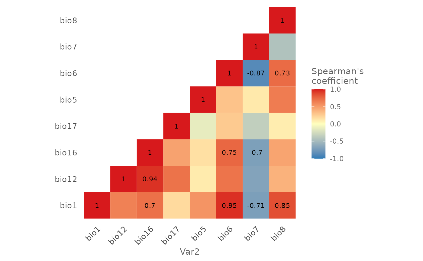
With the function plotCor() you can create an heat map showing the degree of autocorrelation:

plotCor(bg, 
        method = "spearman", 
        cor_th = 0.7)

You can select a different correlation method or set a different correlation threshold. Another useful function is corVar() that instead of creating a heat map prints the pairs of correlated variables according to the given method and correlation threshold:

corVar(bg, 
       method = "spearman", 
       cor_th = 0.7)

Var1	Var2	value
bio1	bio6	0.9513541
bio12	bio16	0.9447559
bio6	bio7	-0.8734498
bio1	bio8	0.8459649
bio16	bio6	0.7471269
bio6	bio8	0.7286723
bio1	bio7	-0.7119135
bio16	bio7	-0.7027568
bio1	bio16	0.7023585

As you can see there are few variables that have a correlation coefficient greater than 0.7 in absolute value.

Remove highly correlated variables

SDMtune implements an algorithm that removes highly correlated variables repeating the following steps:

1. ranks the variables according to the permutation importance or the percent contribution (the second method is available only for Maxent models).
2. checks if the variable ranked as most important is highly correlated with other variables, according to the given method and correlation threshold. If the algorithm finds correlated variables it moves to the next step, otherwise checks the other variables in the rank;
3. performs a leave one out Jackknife test among the correlated variables;
4. remove the variable that decreases the less the model performance when removed, according to the given metric on the training dataset.

The process is repeated until the remaining variables have a correlation coefficient lower than the provided correlation threshold. In the next example we remove the variables that have a Spearman correlation coefficient \(|r_s|\leq0.7\) and checking the AUC on the training dataset (we use only one permutation to save time but you are free to increase this value). If you use RStudio, the function creates an interactive real-time chart in the viewer pane. Run the following code and hover over the chart during the execution of the function to get extra information:

selected_variables_model <- varSel(maxnet_model, 
                                   metric = "auc", 
                                   test = test, 
                                   bg4cor = bg, 
                                   method = "spearman", 
                                   cor_th = 0.7, 
                                   permut = 1)

#> ✔ The variables bio16, bio6, bio7, and bio8 have been removed

As you can see some variables have been removed. The output of the function is the model trained with the selected variables:

selected_variables_model
#> 
#> ── Object of class: <SDMmodel> ──
#> 
#> Method: Maxnet
#> 
#> ── Hyperparameters
#> • fc: "lqph"
#> • reg: 1
#> 
#> ── Info
#> • Species: Virtual species
#> • Presence locations: 320
#> • Absence locations: 5000
#> 
#> ── Variables
#> • Continuous: "bio1", "bio12", "bio17", and "bio5"
#> • Categorical: "biome"

Try yourself

Remove highly correlated variables using the default_model, ranking the variables with the percent contribution and using the AICc as evaluation metric. Check the help of the function varSel() and highlight the next cell to see the solution:

# You need to pass the env argument for the AICc and the use_pc argument to use the percent contribution
selected_variables_model <- varSel(default_model, 
                                   metric = "aicc", 
                                   bg4cor = bg, 
                                   method = "spearman", 
                                   cor_th = 0.7, 
                                   env = predictors, 
                                   use_pc = TRUE)

Remove variables with low importance

There are cases in which a model has some environmental variables ranked with very low contribution and you may want to remove some of them to reduce the model complexity. SDMtune offers two different strategies implemented in the function reduceVar(). We will use the maxnet_model trained with all the variables. Let’s first check the permutation importance (we use only one permutation to save time):

varImp(maxnet_model, 
       permut = 1)

Variable	Permutation_importance
bio1	56.1
bio8	19.5
bio17	6.3
biome	4.7
bio12	3.5
bio5	3.5
bio7	3.2
bio6	1.6
bio16	1.5

We will use the function reduceVar() only for demonstration purpose. In the first example we want to remove all the environmental variables that have a permutation importance lower than 6%, no matter if the model performance decreases. The function removes the last ranked environmental variable, trains a new model and computes a new rank. The process is repeated until all the remaining environmental variables have an importance greater than 6%:

cat("Testing AUC before: ", auc(maxnet_model, test = test))
#> Testing AUC before:  0.8505888

reduced_variables_model <- reduceVar(maxnet_model, 
                                     th = 6, 
                                     metric = "auc", 
                                     test = test, 
                                     permut = 1)
#> ✔ The variables bio16, bio6, bio7, bio5, bio17, and biome have been removed

cat("Testing AUC after: ", auc(reduced_variables_model, test = test))
#> Testing AUC after:  0.8520787

In the second example we want to remove the environmental variables that have a permutation importance lower than 15% only if removing the variables the model performance does not decrease, according to the given metric. In this case the function performs a leave one out Jackknife test and remove the environmental variables in a step-wise fashion as described in the previous example, but only if the model performance doesn’t drop:

cat("Testing AUC before: ", auc(maxnet_model, test = test))
#> Testing AUC before:  0.8505888

reduced_variables_model <- reduceVar(maxnet_model, 
                                     th = 15, 
                                     metric = "auc", 
                                     test = test, 
                                     permut = 1, 
                                     use_jk = TRUE)
#> ✔ The variables bio16, bio6, bio5, bio12, biome, and bio8 have been removed

cat("Testing AUC after: ", auc(reduced_variables_model, test = test))
#> Testing AUC after:  0.8533188

As you can see in this case several variables have been removed and the AUC in the testing dataset didn’t decrease.

Try yourself

Reduce the number of variables using the model trained with the cross validation and using as metric the TSS. Highlight the following cell for the solution:

# You need to pass TRUE to the test argument
selected_variables_model <- reduceVar(cv_model, 
                                      th = 6, 
                                      metric = "tss", 
                                      test = TRUE, 
                                      permut = 1)

Conclusion

In this article you have learned:

• how to explore the correlation between the environmental variables;
• a possible approach to remove highly correlated environmental variables;
• two possible methods to remove environmental variables with low importance.

In the next article you will learn how to tune the model hyperparameters.